AMLR Auto Machine Learning Report
Architecture

AMRL The Scientist (www.thescientist.com.br)

Exploratory Data Analisys

In statistics, exploratory data analysis is an approach to analyzing data sets to summarize their main characteristics, often using statistical graphics and other data visualization methods. A statistical model can be used or not, but primarily EDA is for seeing what the data can tell us beyond the formal modeling or hypothesis testing task. Exploratory data analysis was promoted by John Tukey to encourage statisticians to explore the data, and possibly formulate hypotheses that could lead to new data collection and experiments. EDA is different from initial data analysis (IDA), which focuses more narrowly on checking assumptions required for model fitting and hypothesis testing, and handling missing values and making transformations of variables as needed. EDA encompasses IDA.

Wikipedia


Preliminar Results

Data Set
Shape 891 / 12
Classes 2
Classes Found ['Yes' 'No']
Duplicated none
Excluded Features:
Feature Freq
PassengerId 1.0
Name 1.0
Ticket 0.7643097643097643
column dtype not_null percent
Survived object 891 0.0
Pclass int64 891 0.0
Sex object 891 0.0
Age float64 714 0.1987
SibSp int64 891 0.0
Parch int64 891 0.0
Fare float64 891 0.0
Cabin object 204 0.771
Embarked object 889 0.0022
Several characteristics define a data set's structure and properties. These include the number and types of the attributes or variables, and various statistical measures applicable to them, such as standard deviation and kurtosis. The values may be numbers, such as real numbers or integers, for example representing a person's height in centimeters, but may also be nominal data (i.e., not consisting of numerical values), for example representing a person's ethnicity. More generally, values may be of any of the kinds described as a level of measurement. For each variable, the values are normally all of the same kind. However, there may also be missing values, which must be indicated in some way.

Wikipedia

Regression Analisys

                            OLS Regression Results                            
==============================================================================
Dep. Variable:               Survived   R-squared:                       0.384
Model:                            OLS   Adj. R-squared:                  0.378
Method:                 Least Squares   F-statistic:                     68.72
Date:                Sun, 21 Mar 2021   Prob (F-statistic):           1.34e-87
Time:                        11:35:42   Log-Likelihood:                -406.12
No. Observations:                 891   AIC:                             830.2
Df Residuals:                     882   BIC:                             873.4
Df Model:                           8                                         
Covariance Type:            nonrobust                                         
==============================================================================
                 coef    std err          t      P>|t|      [0.025      0.975]
------------------------------------------------------------------------------
Intercept      0.2163      0.107      2.024      0.043       0.007       0.426
Pclass         0.1564      0.023      6.754      0.000       0.111       0.202
Sex            0.5156      0.029     18.085      0.000       0.460       0.572
Age            0.0026      0.001      3.166      0.002       0.001       0.004
SibSp          0.0382      0.013      2.888      0.004       0.012       0.064
Parch          0.0070      0.018      0.382      0.702      -0.029       0.043
Fare          -0.0004      0.000     -1.189      0.235      -0.001       0.000
Cabin          0.0002      0.000      0.424      0.671      -0.001       0.001
Embarked       0.0247      0.021      1.179      0.239      -0.016       0.066
==============================================================================
Omnibus:                       42.170   Durbin-Watson:                   1.892
Prob(Omnibus):                  0.000   Jarque-Bera (JB):               47.161
Skew:                          -0.561   Prob(JB):                     5.74e-11
Kurtosis:                       3.109   Cond. No.                     1.21e+03
==============================================================================

Notes:
[1] Standard Errors assume that the covariance matrix of the errors is correctly specified.
[2] The condition number is large, 1.21e+03. This might indicate that there are
strong multicollinearity or other numerical problems.


In statistical modeling, regression analysis is a set of statistical processes for estimating the relationships between a dependent variable (often called the 'outcome variable') and one or more independent variables (often called 'predictors', 'covariates', or 'features'). The most common form of regression analysis is linear regression, in which one finds the line (or a more complex linear combination) that most closely fits the data according to a specific mathematical criterion.

Wikipedia

Balance Classes
Unbalance Classes
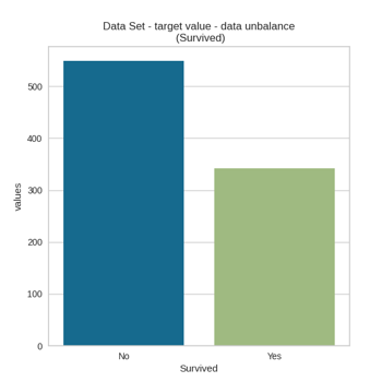
The accuracy paradox is the paradoxical finding that accuracy is not a good metric for predictive models when classifying in predictive analytics. This is because a simple model may have a high level of accuracy but be too crude to be useful. For example, if the incidence of category A is dominant, being found in 99% of cases, then predicting that every case is category A will have an accuracy of 99%. Precision and recall are better measures in such cases. The underlying issue is that there is a class imbalance between the positive class and the negative class. Prior probabilities for these classes need to be accounted for in error analysis. Precision and recall help, but precision too can be biased by very unbalanced class priors in the test sets.

Wikipedia

Correlation of the Features
Correlation
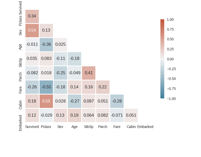
In statistics, correlation or dependence is any statistical relationship, whether causal or not, between two random variables or bivariate data. In the broadest sense correlation is any statistical association, though it commonly refers to the degree to which a pair of variables are linearly related.

Wikipedia

Detecting Multicollinearity with VIF
cols vif significant
Pclass 17.961410161938964 high
Sex 12.93806509064671 high
Age 3.3903676913387613 attention
SibSp 1.5729629081657512 moderate
Parch 1.6246468770706608 moderate
Fare 1.9201681831506432 moderate
Cabin 25.31643019376367 high
Embarked 23.504359385472068 high
In statistics, multicollinearity (also collinearity) is a phenomenon in which one predictor variable in a multiple regression model can be linearly predicted from the others with a substantial degree of accuracy. In this situation, the coefficient estimates of the multiple regression may change erratically in response to small changes in the model or the data. Multicollinearity does not reduce the predictive power or reliability of the model as a whole, at least within the sample data set; it only affects calculations regarding individual predictors. That is, a multivariate regression model with collinear predictors can indicate how well the entire bundle of predictors predicts the outcome variable, but it may not give valid results about any individual predictor, or about which predictors are redundant with respect to others.

Wikipedia

Residual Analysis
qqplot hist
In statistics and optimization, errors and residuals are two closely related and easily confused measures of the deviation of an observed value of an element of a statistical sample from its "theoretical value". The error (or disturbance) of an observed value is the deviation of the observed value from the (unobservable) true value of a quantity of interest, and the residual of an observed value is the difference between the observed value and the estimated value of the quantity of interest.

Wikipedia

Grid - Hyperparameter optimization

In machine learning, hyperparameter optimization or tuning is the problem of choosing a set of optimal hyperparameters for a learning algorithm. A hyperparameter is a parameter whose value is used to control the learning process. By contrast, the values of other parameters (typically node weights) are learned.

Wikipedia

AutoML - Results The models are classified by a standard metric based on the type of problem (the second column of the scoreboard). In binary classification problems, this metric is AUC, and in classification problems in several classes, the metric is the average error per class. In regression problems, the standard classification metric is deviation.

model_id auc logloss aucpr mean_per_class_error training_time_ms
StackedEnsemble_AllModels_AutoML_20210321_113603 0.8617742551566081 0.4331629263598107 0.8835750273317714 0.205532212885154 523
StackedEnsemble_BestOfFamily_AutoML_20210321_113603 0.8554664289958408 0.440849822006415 0.8788874967600675 0.2294796706561412 378
DeepLearning_grid__1_AutoML_20210321_113603_model_1 0.8552966641201936 0.5097096623401154 0.8821560261703341 0.2437505305152364 8856
XGBoost_1_AutoML_20210321_113603 0.8531799083269672 0.4492998872547507 0.8726242559396336 0.2206731177319413 297
XGBoost_grid__1_AutoML_20210321_113603_model_7 0.8476254138018845 0.4571305830675741 0.870164877389272 0.2685255920550038 198
DRF_1_AutoML_20210321_113603 0.8475776674306086 0.6854196051603384 0.8584765041999396 0.2509018759018759 492
DeepLearning_grid__1_AutoML_20210321_113603_model_2 0.8452434003904592 0.5154685972340852 0.8742553433025232 0.215219421101774 57170
XGBoost_3_AutoML_20210321_113603 0.8449197860962567 0.4697695248370234 0.8541170350152238 0.2211081402257873 120
XGBoost_grid__1_AutoML_20210321_113603_model_4 0.8445006790595025 0.4822409965419599 0.8657805553007771 0.2404082845259316 191
DeepLearning_grid__3_AutoML_20210321_113603_model_1 0.8442407265936678 0.5046830052243463 0.8729386081950662 0.246254562431033 18953
XGBoost_grid__1_AutoML_20210321_113603_model_2 0.840219421101774 0.4581873370268132 0.8546380317505627 0.2517188693659282 155
DeepLearning_grid__2_AutoML_20210321_113603_model_1 0.8389727102962398 0.5072303956402726 0.8604405805286884 0.2139567948391477 13516
XGBoost_2_AutoML_20210321_113603 0.8386013496307614 0.4644141617396364 0.8588804592849213 0.2298934725405314 233
XGBoost_grid__1_AutoML_20210321_113603_model_3 0.838044308632544 0.4732102824915125 0.8558593230810595 0.2462757830404889 176
XRT_1_AutoML_20210321_113603 0.8361450640862406 0.4951652618251404 0.8728974374939512 0.2186359392241745 359
XGBoost_grid__1_AutoML_20210321_113603_model_1 0.8356676003734828 0.5130622224898123 0.860814893148308 0.2777777777777778 155
XGBoost_grid__1_AutoML_20210321_113603_model_5 0.8354129530600118 0.464244363776416 0.8565953317621243 0.2462651727357609 110
XGBoost_grid__1_AutoML_20210321_113603_model_6 0.8351211696799933 0.4714487700737709 0.8623428704702091 0.2710296239708005 147
DeepLearning_1_AutoML_20210321_113603 0.8334871827518887 0.4810777653224323 0.8588388140567175 0.2802818096935744 250
GLM_1_AutoML_20210321_113603 0.8332749766573296 0.463766461906979 0.8659859728453491 0.2483554027671674 486
DeepLearning_grid__2_AutoML_20210321_113603_model_2 0.8239750445632799 0.6421969902824427 0.8552718211552578 0.2349439775910364 336006
DeepLearning_grid__3_AutoML_20210321_113603_model_2 0.8076298701298701 0.5910237364231313 0.8450830089436178 0.2815444359562006 360689

Partial dependence plot (PDP) gives a graphical depiction of the marginal effect of a variable on the response. The effect of a variable is measured in change in the mean response. PDP assumes independence between the feature for which is the PDP computed and the rest.

An Individual Conditional Expectation (ICE) plot gives a graphical depiction of the marginal effect of a variable on the response. ICE plots are similar to partial dependence plots (PDP); PDP shows the average effect of a feature while ICE plot shows the effect for a single instance. This function will plot the effect for each decile. In contrast to the PDP, ICE plots can provide more insight, especially when there is stronger feature interaction.

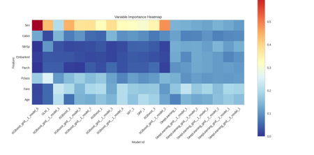
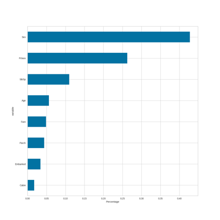
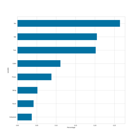
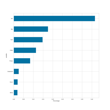
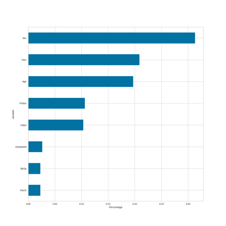
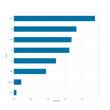
Variable Importance by Model

Variable Importance Model

AML - Partial Dependence

Ensemble - (ICE) Individual Condition Expectation

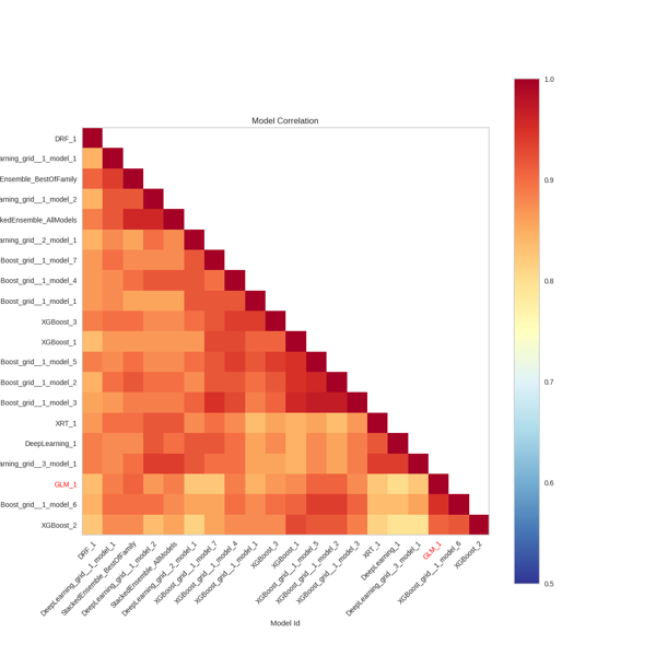
Correlation Heatmap by Model

AML Correlation Model

Model Performance

Analytical Performance Modeling

Analytical Performance Modeling is a method to model the behaviour of a system in a spreadsheet. It is used in Software performance testing. It allows evaluation of design options and system sizing based on actual or anticipated business usage. It is therefore much faster and cheaper than performance testing, though it requires thorough understanding of the hardware platforms

Wikipedia


Comparative Metrics Table

Algo Overall ACC Kappa Overall RACC SOA1(Landis & Koch) SOA2(Fleiss) SOA3(Altman) SOA4(Cicchetti) SOA5(Cramer) SOA6(Matthews) TNR Macro TPR Macro FPR Macro FNR Macro PPV Macro ACC Macro F1 Macro TNR Micro FPR Micro TPR Micro FNR Micro PPV Micro F1 Micro Scott PI Gwet AC1 Bennett S Kappa Standard Error Kappa 95% CI Chi-Squared Phi-Squared Cramer V Chi-Squared DF 95% CI Standard Error Response Entropy Reference Entropy Cross Entropy Joint Entropy Conditional Entropy KL Divergence Lambda B Lambda A Kappa Unbiased Overall RACCU Kappa No Prevalence Mutual Information Overall J Hamming Loss Zero-one Loss NIR P-Value Overall CEN Overall MCEN Overall MCC RR CBA AUNU AUNP RCI Pearson C CSI ARI Bangdiwala B Krippendorff Alpha
GLM 0.8125 0.5741 0.5598 Moderate Intermediate to Good Moderate Fair Strong Moderate 0.7647 0.7647 0.2353 0.2353 0.8697 0.8125 0.7794 0.8125 0.1875 0.8125 0.1875 0.8125 0.8125 0.5587 0.674 0.625 0.0701 0.7115 62.6294 0.3914 0.6256 1.0 0.873 0.0309 0.7579 0.9672 1.0793 1.4094 0.4422 0.1121 0.1429 0.5238 0.5587 0.5751 0.625 0.3157 0.6466 0.1875 30.0 0.6062 0.0 0.4703 0.3361 0.6256 80.0 0.6538 0.7647 0.7647 0.3264 0.5304 0.6344 0.3792 0.7238 0.5601
Random Forest 0.8312 0.6311 0.5425 Substantial Intermediate to Good Good Good Strong Moderate 0.8024 0.8024 0.1976 0.1976 0.8438 0.8312 0.8138 0.8312 0.1687 0.8312 0.1687 0.8312 0.8312 0.6276 0.6914 0.6625 0.0647 0.758 66.5292 0.4158 0.6448 1.0 0.8893 0.0296 0.8813 0.9672 0.9959 1.5317 0.5645 0.0287 0.4375 0.5714 0.6276 0.5469 0.6625 0.3168 0.6899 0.1688 27.0 0.6062 0.0 0.5502 0.4227 0.6448 80.0 0.7396 0.8024 0.8024 0.3275 0.5419 0.6462 0.4319 0.7233 0.6287
GBM 0.8375 0.6499 0.5359 Substantial Intermediate to Good Good Good Strong Moderate 0.8159 0.8159 0.1841 0.1841 0.8404 0.8375 0.8242 0.8375 0.1625 0.8375 0.1625 0.8375 0.8375 0.6484 0.6979 0.675 0.0628 0.773 68.8252 0.4302 0.6559 1.0 0.8947 0.0292 0.9162 0.9672 0.9795 1.5561 0.5889 0.0124 0.5094 0.5873 0.6484 0.5378 0.675 0.3273 0.7039 0.1625 26.0 0.6062 0.0 0.5615 0.4367 0.6559 80.0 0.773 0.8159 0.8159 0.3384 0.5484 0.6563 0.4499 0.725 0.6495
xGBoost 0.8562 0.6912 0.5345 Substantial Intermediate to Good Good Good Strong Moderate 0.8369 0.8369 0.1631 0.1631 0.8597 0.8562 0.8451 0.8562 0.1438 0.8562 0.1438 0.8562 0.8562 0.6901 0.7319 0.7125 0.0596 0.808 77.5677 0.4848 0.6963 1.0 0.9106 0.0277 0.9224 0.9672 0.9771 1.5158 0.5486 0.01 0.5741 0.6349 0.6901 0.5361 0.7125 0.3738 0.7339 0.1438 23.0 0.6062 0.0 0.5219 0.4079 0.6963 80.0 0.7975 0.8369 0.8369 0.3865 0.5714 0.6966 0.5026 0.7534 0.6911
Deep Learning 0.6875 0.3597 0.512 Fair Poor Fair Poor Moderate Weak 0.6838 0.6838 0.3162 0.3162 0.6778 0.6875 0.679 0.6875 0.3125 0.6875 0.3125 0.6875 0.6875 0.358 0.3911 0.375 0.0751 0.5069 20.9202 0.1308 0.3616 1.0 0.7593 0.0366 0.9909 0.9672 0.9746 1.8623 0.8951 0.0074 0.2958 0.2063 0.358 0.5132 0.375 0.0958 0.5164 0.3125 50.0 0.6062 0.0205 0.8251 0.6377 0.3616 80.0 0.6463 0.6838 0.6838 0.099 0.34 0.3616 0.135 0.4874 0.3601

The Best Algorithms

Description RF GLM GBM XGB DL
overall 4.48333 3.86667 4.48333 4.48333 2.38333
class 8.3 8.4 7.8 8.3 5.6

The best name: Winners: RF - GBM - XGB
Confusion matrices are too close and the best one can not be recognized.


Gradient Linear Estimator
Confusion Matrix
Description precision recall f1-score support
Yes 0.9714 0.5397 0.6939 63.0
No 0.768 0.9897 0.8649 97.0
accuracy 0.8125 0.8125 0.8125 0.8125
macro avg 0.8697 0.7647 0.7794 160.0
weighted avg 0.8481 0.8125 0.7975 160.0
Feature Importance
Feature Importance

Dynamic Random Forest
Confusion Matrix
Description precision recall f1-score support
Yes 0.875 0.6667 0.7568 63.0
No 0.8125 0.9381 0.8708 97.0
accuracy 0.8312 0.8312 0.8312 0.8312
macro avg 0.8438 0.8024 0.8138 160.0
weighted avg 0.8371 0.8312 0.8259 160.0
Feature Importance
Feature Importance

Gradient Boost Machine
Confusion Matrix
Description precision recall f1-score support
Yes 0.8491 0.7143 0.7759 63.0
No 0.8318 0.9175 0.8725 97.0
accuracy 0.8375 0.8375 0.8375 0.8375
macro avg 0.8404 0.8159 0.8242 160.0
weighted avg 0.8386 0.8375 0.8345 160.0
Feature Importance
Feature Importance

XGBoost
Confusion Matrix
Description precision recall f1-score support
Yes 0.8704 0.746 0.8034 63.0
No 0.8491 0.9278 0.8867 97.0
accuracy 0.8562 0.8562 0.8562 0.8562
macro avg 0.8597 0.8369 0.8451 160.0
weighted avg 0.8574 0.8562 0.8539 160.0
Feature Importance
Feature Importance

Deep Learning
Confusion Matrix
Description precision recall f1-score support
Yes 0.5915 0.6667 0.6269 63.0
No 0.764 0.701 0.7312 97.0
accuracy 0.6875 0.6875 0.6875 0.6875
macro avg 0.6778 0.6838 0.679 160.0
weighted avg 0.6961 0.6875 0.6901 160.0
Feature Importance
Feature Importance